Sound Search by Vocal Imitation
Search Algorithms
We proposed three approaches to answer the question of sound search by vocal imitation. One supervised learning model and two unsupervised learning models named IMISOUND and IMINET, respectively.
1. Supervised SAE Model
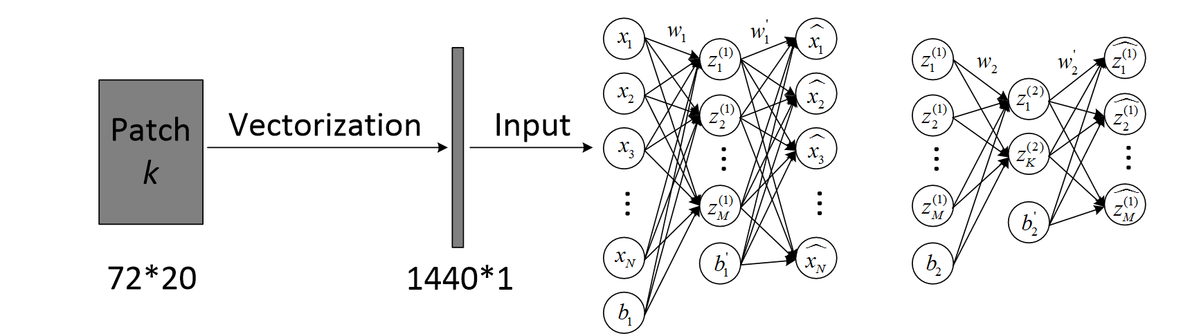
Each vocal imitation and sound recording is downsampled, converted to Constant-Q Transform spectrogram, and then segmented into overlapping patches. Then a two-hidden-layer stacked auto-encoder (SAE) is applied to learn features automatically from a set of vocal imitations in an unsupervised way (see Figure 1.1).
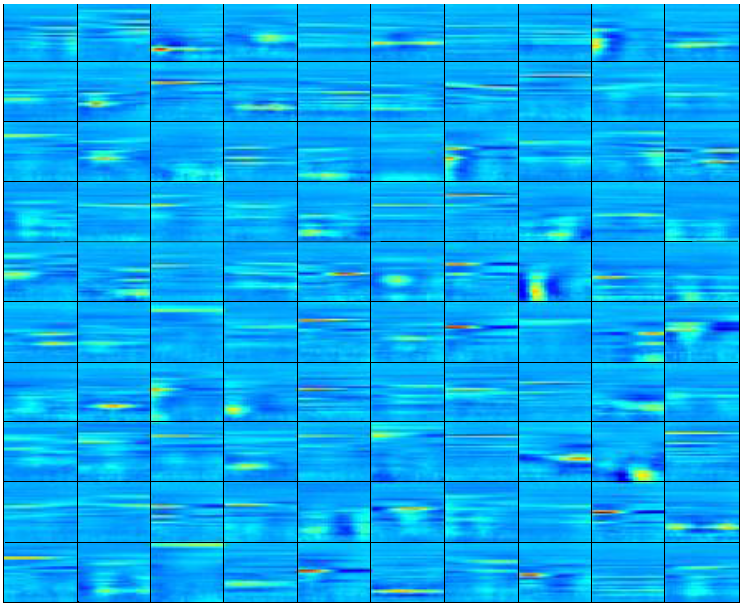
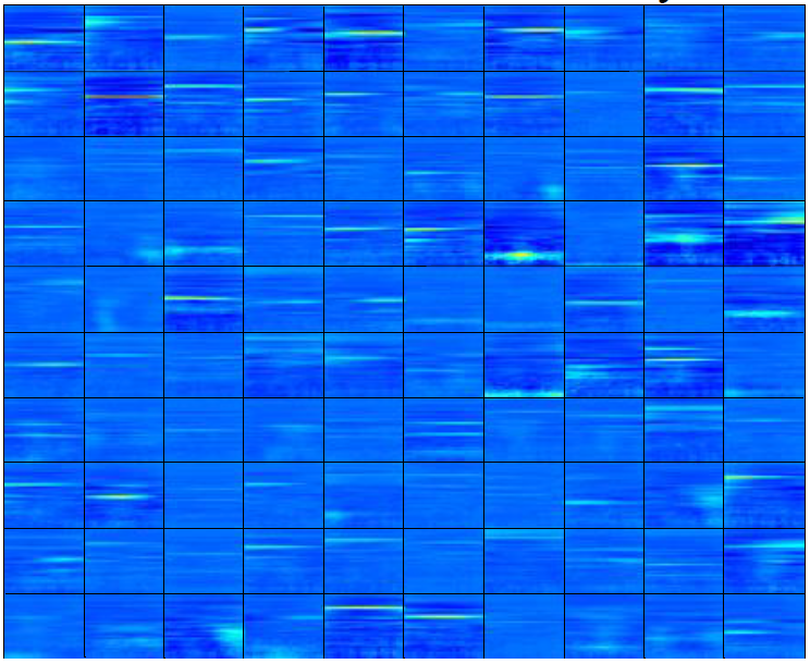
Features learned in this way characterize acoustic aspects that human often imitate. We set the number of neurons in the first and second hidden layers to 500 and 100, respectively. Weights connected from the previous layer to each neuron compose a feature. Therefore, there are 500 and 100 features in the first and second hidden layers, respectively. Figure 2. visualizes these features. Due to the limited space, we only display the first 100 out of 500 features in the first hidden layer. Notice that the first hidden layer extracts features that act as building blocks of the CQT spectrogram. The feature for each neuron in the second hidden layer is obtained by a weighted linear combination of features of the first hidden layer neurons to which it is strongly connected. These features are more abstract.
In the supervised approach to recognize vocal imitations, for each sound concept, we assume that a number of vocal imitations are available for training. A multi-class Support Vector Machine (SVM) is employed to learn to discriminate vocal imitations of different sound concepts. Then the classifier is able to classify a new vocal imitation to one of these trained sound concepts. For a new vocal imitation whose underlying sound concept is unknown, the multi-class SVM classifies each patch of it to one of the trained sound concepts. Then majority vote is conducted to obtain the recording-level classification.
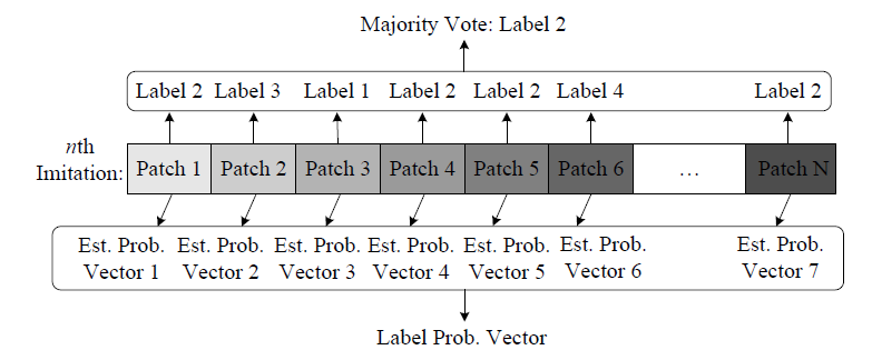
We also obtain a probabilistic classification output, showing the probability (confidence) that the vocal imitation patch belongs to each of the trained sound concepts. We then sort sound concepts according to their classification probabilities from high to low, and return sounds of highly-ranked concepts. For sound concepts at the recording level, we average the probability output over all the patches in one imitation, and then sort sound concepts according to the averaged classification probability from high to low. Again, sounds of highly-ranked concepts can be retrieved. Figure 1.3 illustrates the overall process.
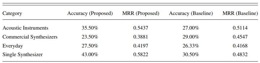
For the sound search performance, we compare the supervised system using automatic feature learning to a baseline system using 472-d hand-crafted features including global descriptors and timevarying descriptors from each vocal imitation by the Timbre Toolbox. From Table 1.1 we found: (1) Both the proposed and baseline systems achieve significantly higher classification performance than random guesses. (2) The average classification and sound retrieval performance of the proposed system outperforms that of the baseline in most categories.
2. IMISOUND
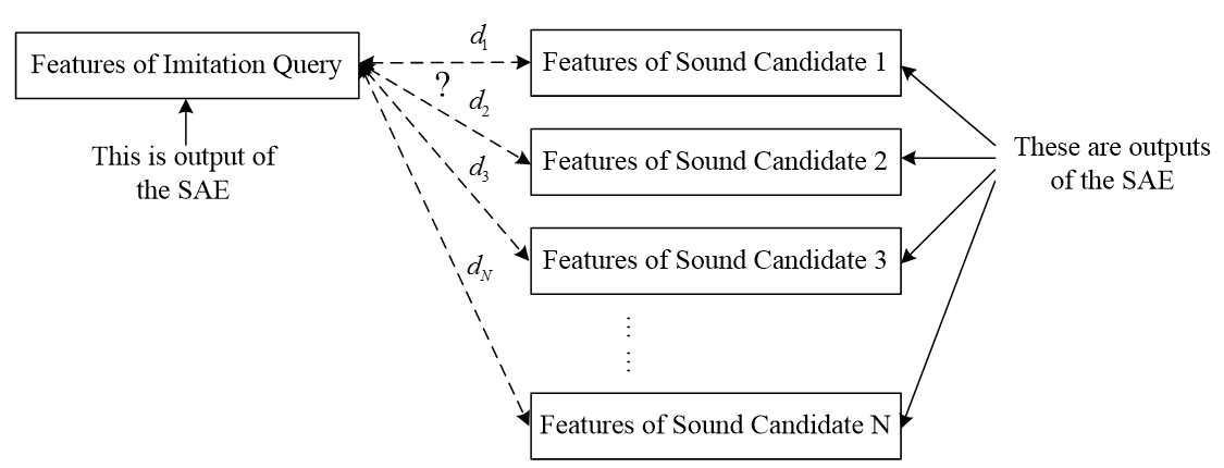
To make sound retrieval more flexible and independent of the existence of training vocal imitations of sounds, we then design an unsupervised system named IMISOUND. Again, this system uses the automatically learned representations for vocal imitations. It also represents sounds in the library with this representation, mapping sounds to the same feature space as vocal imitations. It then calculates the distances between the imitation query and each sound in the library and retrieves the closest sounds (see Figure 2.1).
So now both the imitation query and the target sound are represented by a sequence of vectors. We adopt the combined distance of: (1) Dynamic Time Warping (DTW), and (2) symmetric K-L divergence, to describe the temporal evolution and probability distribution between the imitation query and target sound. Cosine distance is also adopted in our system.
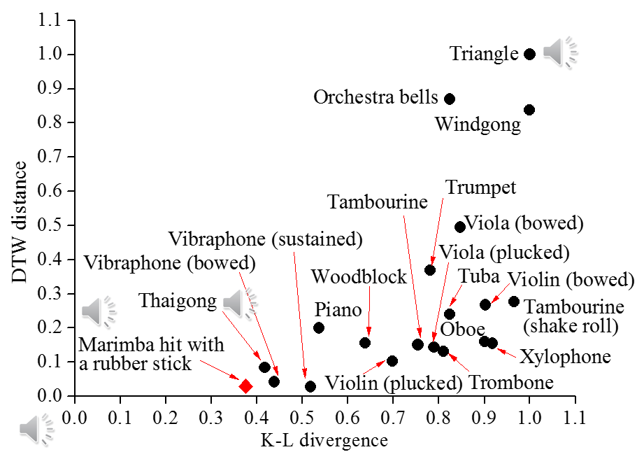
Figure 2.2 shows a 2-d plot illustrating the distances between a vocal imitation and sound candidate of different acoustics. We see that the target sound “Marimba hit with a rubber mallet” as well as the similar percussive sound “Thai gong” are the closest to the origin (the vocal imitation) in this 2-d space.
Demonstration: Distances between a vocal imitation and sound candidates of different acoustic instruments.
Vocal imitation of “Marimba hit with a rubber stick”:
Sound concept recording of “Marimba hit with a rubber stick”:
Sound concept recording of “Thaigong”:
Sound concept recording of “Triangle”:
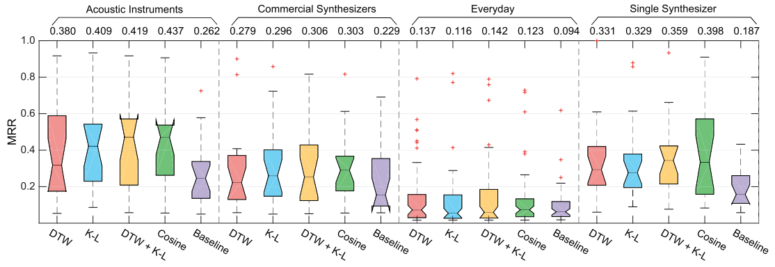
For the sound search performance, we compare four versions of the proposed system and a baseline system. Three out of the four versions use patch level distances: DTW distance, K-L divergence, and their combination. The fourth version uses cosine distance in the recording level. We still adopt Timbre Toolbox as hand-picking features for the baseline method to calculate cosine distance.
From Figure 2.3 we found: (1) All four versions of the proposed system (the first four boxes in each category panel) outperform the baseline system in all categories. (2) The four versions of the proposed system do not show much difference.
3. Siamese Style Model: SYMM-IMINET
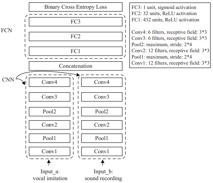
The feature representation and matching algorithm in IMISOUND were designed separately. So we further propose another neural network model called IMINET for sound search by vocal imitation that jointly optimizes feature learning and the matching algorithm. As shown in Figure 3.1, IMINET is a Convolutional Semi-Siamese Network (CSN) that contains (1) two Convolutional Neural Network (CNN) towers for feature learning for vocal imitations (query) and sound recordings (candidate) respectively; and (2) a Fully Connected Network (FCN) for feature learning that classifies the query-candidate feature concatenations into positive and negative pairs.
In IMINET, each tower of the Siamese network is a Convolutional Neural Network(CNN) with 4 convolutional layers. We propose three configurations when designing the convolutional towers:
(1) Tied-weights: The two towers share the exactly same weights and biases in all layers.
(2) Untied-weights: The two towers do not share weights and biases at all, although their structures are the same. This allows the two towers to be tuned for the vocal imitation and sound recordings independently.
(3) Partially-tied-weights: The weights and biases in the two towers are not shared for Conv1 and Conv2 layers, but are shared for Conv3 and Conv4 layers.
After the features from the two towers are extracted, they are flattened, concatenated, and fed into a 3-layer Fully Connected Network (FCN). FC3 uses the sigmoid activation function to squash the output value between 0 and 1, which is viewed as the probability indicating whether the imitation-recording pair is a positive pair (i.e., correct match). The FCN is a metric learning network that learns the similarity between vocal imitations and sound recordings from positive and negative training pairs. Compared to common distance/similarity measures, this metric/similarity is learned together with the feature representations of the vocal imitations and sound recordings, likely leading to a better retrieval performance.
For sound search, the imitation query is paired with each sound candidate in the library and we use IMINET to calculate its likelihood of being a positive pair. Let the likelihood for the i-th sound candidate be L_csn(i). We then rank all sound candidates according to their likelihood from high to low and return the top ones to the user.
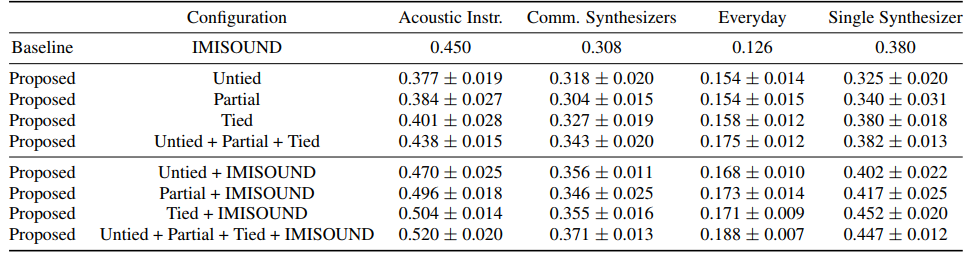
Table 3.1 shows performance comparisons of different configurations of the proposed IMINET, different fusing strategies, and the baseline method from IMISOUND. We found: (1) From untied to partially-tied to tied configurations of IMINET, the MRR increasing trend is observed in all categories. (2) The best performing IMINET configuration, Tied, outperforms IMISOUND on two categories (Commercial Synthesizers and Everyday), underperforms on the Acoustic Instrument category, and achieves comparable performance on the Single Synthesizer category. (3) By fusing different configurations of IMINET together, the MRR is better than each configuration itself. (4) By late fusion of the IMISOUND with each IMINET configuration, the MRR is boosted significantly. (5) The highest MRR in general can be achieved by fusing all configurations of IMINET together as well as IMISOUND.
4. Siamese Style Model: TL-IMINET
The partially tied and untied configurations of SYMM-IMINET introduced flexibilities to the feature extraction towers for them to adapt to their respective inputs, their structures, however, are still the same. Hence we extend the idea to allow structural differences between the two CNN towers. We introduce the transfer learning idea to pre-train the two CNN towers on their own relevant external tasks, leading to the TL-IMINET model.
4.1 Model Structure
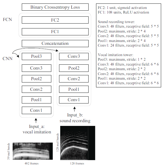
The overall structure of TL-IMINET is shown in Figure 4.1. It is also a Siamese style convolutional neural network, but the structure is not as symmetric as SYMM-IMINET. The recording and imitation towers for feature extraction are adapted from environmental sound classification and spoken language recognition tasks, respectively, hence are asymmetric. The two tower weights and biases are initialized by pre-training them on external datasets for these tasks. They are then fine-tuned together with the FC layers on the sound retrieval task. At test time, the sound retrieval procedure is the same as SYMM-IMINET: The network output is a similarity value between an imitation query and an original sound candidate from the search database. Sound candidates with highest similarity values are returned.
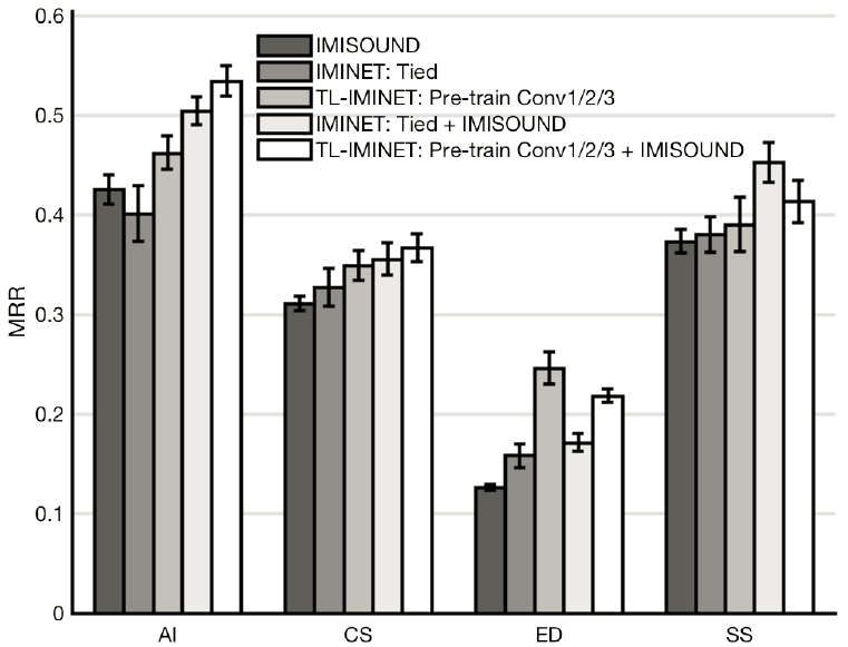
For the sound search performance, we employ the same experimental setup described in SYMM-IMINET. We report the average MRR across 10 runs of the system. In Figure 4.2 we compare it with our previous SYMM-IMINET system with tied configuration, which was the best model on this dataset. It can be seen that without pre-training the CNN towers, TL-IMINET achieves a similar MRR as Tied-IMINET on AI, CS and SS categories, and outperforms Tied-IMINET on ED category. With pre-training, the MRR value is significantly improved across all categories, showing the benefit of transfer learning and that TL-IMINET is the new state of the art based on our previous work.
4.2 Neural Network Interpretation
In order to obtain more insights on how IMINET works, we visualize and sonify the input pattens that maximize the activation of certain neurons in each layer, using the activation maximization approach. As TL-IMINET achieves the best result, we choose TL-IMINET for this analysis. Activation maximization can be done by gradient ascent of the neuron's activation w.r.t. the input from a random initialization, while keeping the trained weights unchanged. After convergence, the updated input spectrogram can be interpreted as what the neuron learns. For better visualization purposes, ReLU activations in TL-IMINET are replaced by leaky ReLU with a slope of 0.3 for negative inputs. This is to prevent the zero gradient issue when the input value to the ReLU activation is negative, which will trap the optimization. We further sonify the generated input magnitude spectrograms by recovering the phase information using the Griffin-Lim algorithm. The visualization for all input patterns and their corresponding sonified waveforms can be accessed via here. Below shows a few representative examples.
a. Imitation Tower
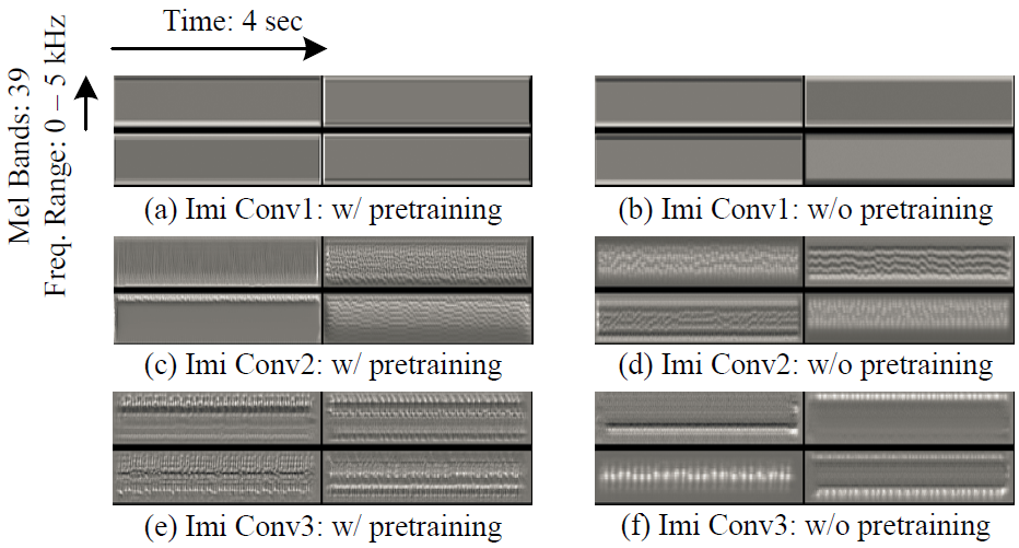
The left and right column of Figure 9 shows the filter visualization of the imitation tower with and without pre-training, respectively. First, taking the top left corner pattern in the left column as an example, the horizontal and vertical dimension represents the number of time frames and frequency bins in mel scale, respectively. Whiter color represents higher energy. Note that first layer (Conv1) neurons learn local features like edges, intermediate layer (Conv2) neurons capture more complicated information such as texture with various directions, while the deepest layer (Conv3) neurons recognize spectrogram-like patterns, with a concentration on different frequency ranges. Second, input patterns visualized with pre-training are generally shaper and contain more finer patterns compared with those without pre-training. This suggests that pre-training on the VoxForge dataset helps the feature extraction tower to pay more attention to spectral details. The sonifications in Conv1 sound like low frequency humming, in Conv2 we hear more spectral components, and in Conv3 delicate birding chirping and water flowing like sounds can be heard.
b. Recording Tower
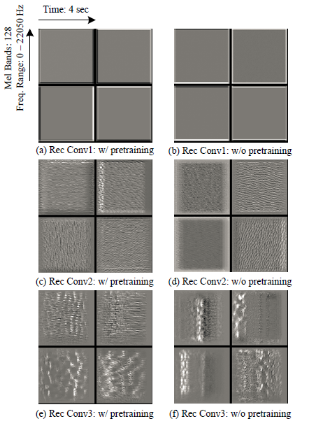
Figure 4.4 shows input patterns that maximally activate several neurons in the original sound recording tower, with and without pre-training. Interesting findings are also observed: First, we discover the same trend of pattern complexity from shallow layers to deep layers, with input patterns from simple and oriented edges to various texture-like patterns, eventually to spectrogram-like complex and hierarchical structures. Second, dissimilar with what we observed earlier in Conv3 of the imitation tower, Conv3 input patterns of the recording tower tend to learn vertical strips besides horizontal patterns. When more complex stimuli are provided, early auditory responses progressively show simple-to-structural periodic patterns along time and frequency directions in auditory spectrograms similar to our visualization results in different neural network layers. For the recording tower sonification, in Conv1 we can hear simple sound patterns like constant pitch and spike, in Conv2 we can hear fast changing patterns in time, and in Conv3 modulated sound effects can be heard.
c. Dense Layers
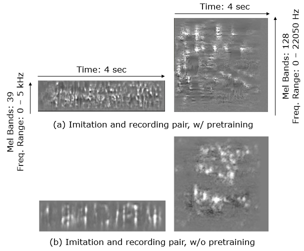
Dense layer filters can be visualized using activation maximization as well. A neuron in a fully connected layer receives a pair of inputs, and the receptive field of each neuron covers the entire input ranges of both the vocal imitation and original recording. Therefore, the neuron is maximally activated by an imitation-original pair instead of an imitation or a original recording alone. Different from the Single-Input-Single-Output (SISO) network structure, in Figure 4.5, we show the maximal activation patterns for 2 representative neurons in layer FC1. The corresponding imitation-original input pattern pairs are shown without and with pre-training TL-IMINET respectively. By pre-training TL-IMINET, more detailed structures from the pairs can be observed compared with the configuration of without pre-training. In both Figure 4.5 (a) and (b), imitation and recording show somewhat similar textures to form a pair. By sonifying the imitation-recording input pattern pairs, we hear that the recovered imitation and original sounds are similar from the aspect of temporal evolution but with timbre being different. The recovered imitation sound is more like natural sound (e.g., generated by certain animals) while the recovered recording sound is similar to a robot voice.
5. Siamese Style Model: CR-IMINET

Figure 5.1. The CR-IMINET model structure.
As shown in Figure 5.1, CR-IMINET contains two identical Convolutional Recurrent Deep Neural Network (CRDNN) towers for feature extraction: One tower receives a vocal imitation (the query) as input. The other receives a sound from the library (the candidate) as input. Each tower outputs a feature embedding. These embeddings are then concatenated and fed into a Fully Connected Network (FCN) for similarity calculation. The final single neuron output from FC2 is the similarity between the query and the candidate. The feature learning and metric learning modules are trained jointly on positive (i.e., related) and negative (i.e., non-related) query-candidate pairs. Through joint optimization, feature embeddings learned by the CRDNNs are better tuned for the FCN's metric learning, compared with isolated feature and metric learning in IMISOUND.
The Siamese (two-tower) and integrated feature and metric learning architecture in the proposed CR-IMINET is inspired by the previous state-of-the-art architecture, TL-IMINET. Differently, TL-IMINET only uses convolutional layers in the feature extraction towers, while CR-IMINET uses both a convolutional layer and a bi-directional GRU (Gated Recurrent Unit) layer. This configuration can better model temporal dependencies in the input log-mel spectrograms. Another difference is that TL-IMINET pre-trains the imitation and recording towers on environmental sound classification and spoken language recognition tasks, respectively, while CR-IMINET does not adopt this pre-training for simplicity thanks to its much smaller model size. Note the "Model Size" column represented by the number of trainable parameters in Table 5.1.
Table 5.1. Model MRR comparisons.

Also in Table 5.1, it can be seen that CR-IMINET outperforms TL-IMINET in terms of MRR. An unpaired t-test shows that this improvement is statistically significant, at the significance level of 0.05 (p = 4.45e-2). An MRR of 0.348 suggests that within the 52 sound candidates in each fold, on average, the target sound is ranked as the top 3 candidate in the returned list. This suggests that CR-IMINET becomes the new state-of-the-art algorithm for sound search by vocal imitation.
6. Interactive Search: Improving Sound Search Using Vocal Imitation Feedback
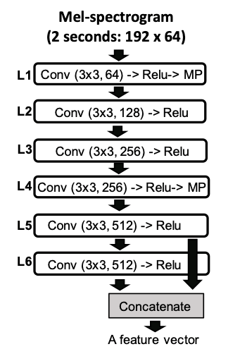
Figure 6.1. The proposed CNN-based
feature extractor.
The performance of a QBV search system depends on the quality of the query. If the query does not provide the right information to sufficiently narrow the search, the target sound(s) will not be top-ranked in the retrieval results. If the search results are not satisfactory, how can a user update the search results? We present a method to update search results when top-ranked items are not relevant: The user provides an additional vocal imitation to illustrate what they do or do not want in the search results. This imitation may either be of some portion of the initial query example, or of a top-ranked (but incorrect) search result.
In order to search for items in the database, the system computes similarities between a query and each item in the database, and return a list of items ordered by the similarity. When user’s vocal imitation is provided, the similarity is updated by two additional similarities between positive/negative vocal imitations and each item in the database. To measure the similarity between real sound and vocal imitation, we used a CNN-based feature extractor (see figure 6.1) where weights on all the layers were taken from VGGish model (Hershey et al., 2017) that has been pre-trained on 8M YouTube dataset. The feature extractor turns every two-second segment of an audio to a feature vector and the final output is formed by averaging feature vectors of all the segments. The similarity between two sounds is calculated using the cosine similarity between their feature vectors.
We measured the performance gain from user’s vocal imitation feedback on two different search tasks: Query-by-Vocalization (QBV) and Query-by-Example (QBE).
6.1 Query-by-Vocalization
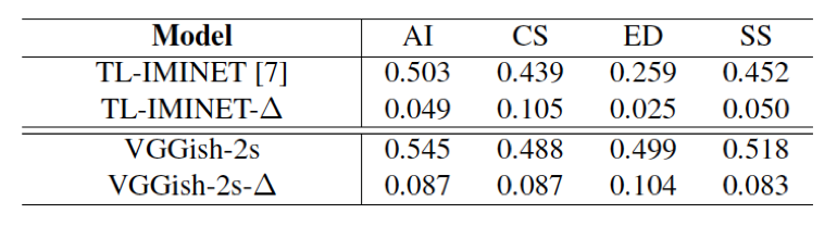
Figure 6.2. MRRs updated by user’s vocal
imitation feedback and performance gain.
To measure the performance gain by imitation feedback on QBV search, we simulated a user’s interaction with the search system as follows. A query (vocal imitation) in the testing set was selected. The reference recordings were ranked by the similarity with the query. If the top-ranked audio was not the target (the reference recording of the vocal imitation query), the initial search rankings were updated using an additional positive query or a vocal imitation of the top-ranked, but incorrect recording (negative example).
The following table shows how search results are improved by additional vocal imitations (one additional positive imitation and one negative imitation) for two different models. We can see that vocal imitation feedback improves MRR on all the models for all the categories of the testing set, which confirms the general efficacy of vocal imitation feedback on QBV.
6.2 Query-by-Example
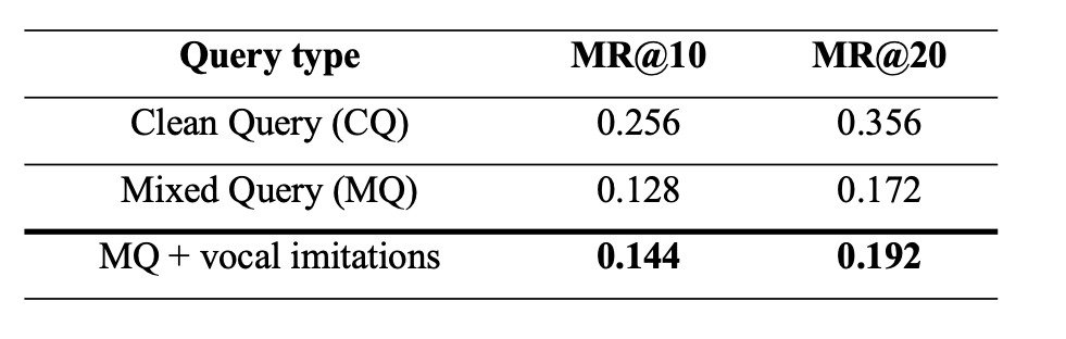
Figure 6.3. Mean Recall@k. There were 301 queries,
each performed on a set of 2,683 items.
We evaluate the effectiveness of vocal imitation feedback when a query containing multiple overlapped sounds is provided to a QBE system. To simulate the scenario, we created a set of Mixed Queries (MQ) each of which contains two different sound events overlapping each other and a set of Clean Queries (CQ) containing only one sound event.
We simulated a user’s interaction with the search system as follows. Given a query (MQ or CQ), the system returns a list of recordings in the testing set (2,683 items) ordered by similarity with the query. If the 5 top-ranked recordings do not include any of relevant recordings (the database has 9 relevant recordings per query), we augment the query using vocal imitations.
To measure its performance, we compute recall within top k items in search results (Recall@K). The following table shows that vocal imitations help to improve the retrieval results.
7. Sound Event Detection Using Point-Labeled Data
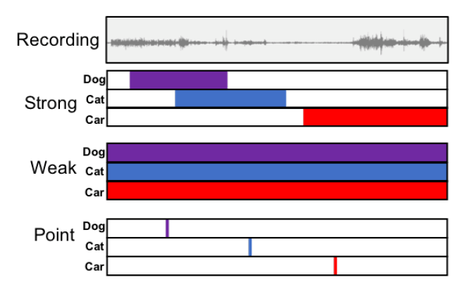
Query by vocalization (QBV) can be considered a kind of Sound Event Detection (SED) in audio scenes. As a byproduct of research done for QBV, we have come upon a novel approach to training deep models for the more general task of SED. This task that has been studied by an increasing number of researchers. Recent SED systems often use deep learning models. Building these systems typically require a large amount of carefully annotated, strongly labeled data, where the exact time-span of a sound event (e.g. the dog bark' starts at 1.2 seconds and ends at 2.0 seconds) in an audio scene (a recording of a city park) is indicated. However, manual labeling of sound events with their time boundaries within a recording is very time-consuming. One way to solve the issue is to collect data with weak labels that only contain the names of sound classes present in the audio file, without time boundary information for events in the file. Therefore, weakly-labeled sound event detection has become popular recently. However, there is still a large performance gap between models built on weakly labeled data and ones built on strongly labeled data, especially for predicting time boundaries of sound events. In this work, we introduce a new type of sound event label, which is easier for people to provide than strong labels. We call them point labels. To create a point label, a user simply listens to the recording and hits the space bar if they hear a sound event ('dog bark'). This is much easier to do than specifying exact time boundaries.
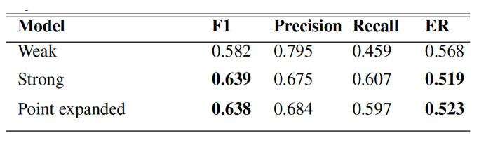
Figure 7.2. Segment-based F1 score, Precision, Recall
(higher is better for all three), and Error Rate (lower is better)
for each model. Segment size is 1 second.
We evaluated the efficacy of point labels for providing a training signal to a deep model for sound event detection. We train models on point-labeled data, weakly-labeled data or strongly-labeled data from URBAN-SED dataset (Salaman, et al., 2017) which contains 10,000 soundscapes. Each file in the dataset is 10 second-long and contains 1 to 9 sound events from 10 different city noise sources. Table 6.2 shows segment-based F1 score with precision and recall and Error Rate for each model. We can see that our point model outperforms the weak model, which shows the point labels help models localize sound events more accurately. Moreover, point model achieved F1 = 0.638 and ER = 0.523 which is nearly identical to our strong model’s score (F1 = 0.639, ER = 0.519). We achieved this performance gain even though we randomly set the positions of point labels, which proves that the point models are robust to the position of point labeling which might vary in real annotation scenario.
Last updated .